DATV in simple terms - Part 2
This article was first published in CQ-TV magazine, issue 209.
We looked last time at how an analogue voltage, which could well be a video or sound signal, could be represented by a stream of numbers. In this part, I hope to explain why converting to digital makes the job of handling the signal so much easier.
It isnt only the fact that digital signals do not normally degrade along their transmission path like analogue ones do that makes them attractive, they are easier to handle in a production environment. Trying to do clever tricks on analogue signals is very difficult, even something as straightforward as cross-fading one picture to another involves sync stripping, locking picture source timings together and then mixing through variable gain amplifiers. Ill explain the simple way its done digitally a little later.
Before getting deeply engrossed in the studio, lets first take a step back and see why digital signals are so much more robust than analogue ones. It all boils down to the ways signals may be degraded as they pass through circuits, cables and over the air.
We can break analogue degradation into two categories, loss of signal integrity and addition of unwanted interference. The signal integrity is impaired whenever it passes through a non-linear circuit, meaning that for a given change of signal entering the circuit, the output changes by a disproportionate amount. Visibly this shows as an error in contrast or brightness and its severity may change with frequency, giving strange shading or smearing effects. If the problem exists near the colour sub-carrier frequency (4.433MHz in PAL, 3.579MHz in NTSC) it can additionally cause loss or excessive colour or even completely wrong colours. The second category, that of unwanted additional signals becoming mixed with the one we want, can be equally troublesome. The most obvious impairment comes from snow in the picture, such as seen when the signal level is weak. This is actually caused by the addition of random voltages to the picture, either from natural sources or from random electron flows in amplifier devices. In most circumstances, the amplification level is turned down when a strong signal is received and this also results in less amplification of the noise source. Undesired effects can also come from reflections or time-shifted versions of the signal being mixed with the original. When the reflection is delayed enough it shows as a ghost image, shadowing its source and displaced to the side. When the delay is smaller, it is no longer visible as a separate image but it can still cause problems due to the ghost adding or subtracting from individual cycles. You have probably noticed that some ghost images look like photographic negatives and if caused by aircraft passing nearby, may alternate from positive to negative. When the delays are very small, the adding of positive reflections and subtraction of negative ones can cause all manner of nasty waveform distortion or even cancellation. Just as over the air signals suffer from this multi-path effect, so can cabled signals if the source and terminating impedances do not match the cable impedance. The effect can be very serious ghosting. The effect is used deliberately sometimes to measure the length of a cable (Time Domain Reflectometry or TDR) as the time delay between a signal and its reflection is proportional to the distance they have travelled and hence the length.
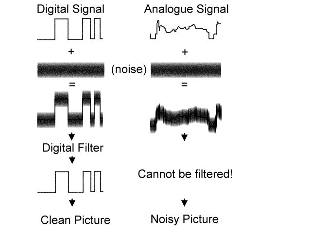
Digital signals have a huge advantage over analogue ones in that they only have two voltage levels instead of the infinite number that analogue has. This virtually removes the need to carry it through linear circuits. The binary bits from the ADC only have two states, a zero or a one. A zero is usually considered to be an absence of voltage while a one is usually a positive voltage, typically 5V. Somewhere between the two there is a threshold, anything below it being considered zero and anything above it considered a one. If 5V is assumed to be the one level and half of that, 2.5V, is assumed to be the threshold, even a signal with 2.4V of noise would still appear to have 100% integrity as it would not cross the threshold from one state to the other. In practice, that would be considered extremely noisy, digital noise levels are usually much lower than that. Even though digital systems are highly immune to noise (fig.3), steps are still taken to minimise the possibility of it interfering. The most common of these is to make the threshold higher than half voltage before assuming a one and lower than half voltage before assuming a zero. In other words, the threshold is no longer fixed, the voltage has to go beyond the half way point to change state either way. This has the effect of cleaning the edges of the signal where the likelihood of noise causing problems is greater during the time rising and falling edges pass through the threshold zone. Not only is a digital signal far less immune to random noise, any reflections in the signal that have lower levels than the threshold are also ignored.
So digital is less prone to distortion and noise, in itself a good reason for using it. Lets now turn to manipulating digital video in various ways and see how much easier it is than in the analogue world. Ive broken the myriads of video effects into just a few categories, most of the more complex tricks are just combinations of these.
Brightness control.
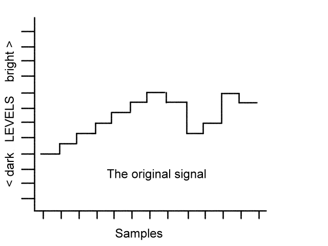
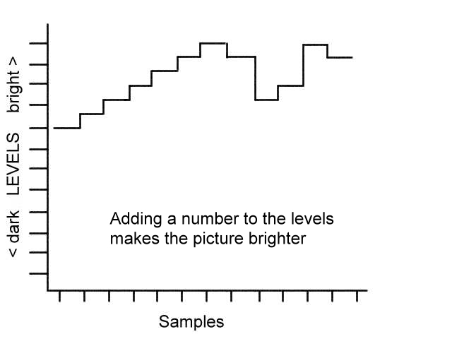
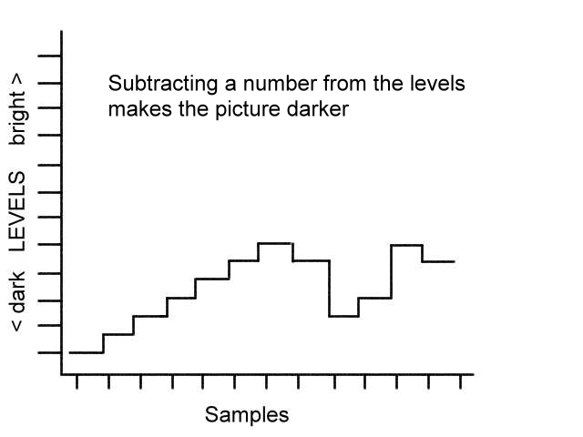
As the picture is made of samples (pixels) and each has a numeric value, simply adding or subtracting from the value will shift the brightness (fig.4abc). The normal value ranged used is 0 - 255 (assuming 8-bit data, its 0-1024 if 10-bit data is used) with higher numbers meaning nearer to peak white. Moving all the pixels up in value makes the whole picture move toward the peak white level. Conversely, if the pixel values are reduced the picture goes darker. Obviously, there is a need to constrain the values so they do not go outside the valid range but thats easy to do.
Figures 4a,4b and 4c
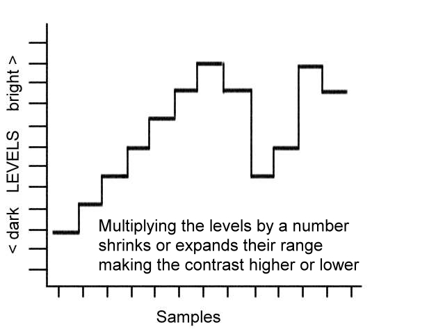
Contrast control.
By contrast we mean the amount of difference between the darkest and lightest parts of the picture. A high contrast means the difference is greater (fig.5). To expand the pixel values so the contrast is higher, all we have to do is multiply each value by a fixed amount. Similarly, dividing causes a contrast reduction.
Hue and saturation.
How these work is somewhat dependant on the way the signals were originally digitised. If the samples represent separate red, green and blue pixel values, the hue can be changed by multiplying (like changing the contrast) each by a different amount. The effect is to unbalance their relative levels and visually cause a colour shift. Saturation is controlled in a similar way but the calculation is a little different as the differences between each colour have to be enhanced by a combination of partially subtracting one from another then multiplying the result to bring the levels back up again. If the samples were digitised from a composite signal, the maths is very complicated and involves a process not too far removed from decoding, enhancing and re-encoding the signal again. I promised no math in part one so Ill leave this aspect for your study elsewhere.
Keying and overlaying.
These are the processes of substituting part of one picture for another. In its simplest form, overlaying, one image, usually a caption or text, is given priority over its background. You will have seen this effect used to put channel logos in the corner of commercial TV broadcasts and to add the names or locations of news reporters into news programmes. Keying is a variation of this where one or more pictures are inserted into another. The effect is frequently used to put weather forecast presenters in front of weather maps. The difference between the two is that one is replacing the background with a new one while the other is switching picture sources at a time decided by either the contents of one of the pictures or a third image called a matte. The matte is usually a black on white fixed image (for example a rectangle the size of the weather map) which decides which image is selected. Black means picture A while white means picture B, obviously the matte image needs to be carefully placed or the picture in picture effect will cut at the wrong places. A variation on the keying theme is colour keying (chroma keying) or luminance keying where the content of one picture, whether colour or brightness is used to switch images. In the analogue world it is quite difficult to distinguish exact levels or colours to operate the signal switch but digitally it is quite easy. Rather than trying to define exact luminance, hues and saturation levels using analogue comparators, we can simply define a range of numbers, the mathematics is very simple.
Cross fading.
Changing from one video source to another can either be an abrupt switch or a gradual fade out of one source as the other fades in. This isnt too difficult to do in analogue circuitry if the signals are synchronised together. However, it involves more than just lowering the level of one source and raising the other. This is because the sync pulses must remain at a contant level throughout. Normally, both sources are stripped of syncs, the video cross faded and then one of the original syncs is re-inserted. Digitally, the same idea is used but the fading in and out is done by numerically reducing one of the samples while applying the same factor to increase the other. For example if sources A and B are multiplied by 0.5, they will both be half level, adding them together will result in full level of a 50/50 mix. Changing so source A is multiplied by 0.25 and source B by 0.75 (thats 1 - 0.25) will give a 25/75 mix in favour of source B.
Synchronising video sources.
The only way to do this using analogue techniques is to genlock the video sources together. A video signal has a visible raster area and synchronising pulses which are not visible but essential to make sure each scan line is in the correct position on the screen. When two or more video sources are mixed, it is essential the sync pulses line up with each other or the one of the pictures will be displaced relative to the other. Normally, this is achieved by using a standard sync pulse generator (SPG) which connects to each of the video sources and keeps them all in time with each other. Doing it digitally is quite different though and the need for genlocking is not as important although still preferable. This is because if the picture is stored as numbers in a memory device it is possible to read them back at a different time. In other words, a degree of time slippage can be catered for by temporarily delaying one of the signals until it falls in line with the other. The memory device takes up the slack. There is a limit to the length of delay that can be used as at some point the memory device will fill up. Thats why it is still important to lock sources if possible, the memory allows for minor time shifts but as it is being written to and read from simultaneously, it will never fill up if the sources are relatively close together.
Without getting bogged down with formulas, here are lines of pseudo code that a computer manipulating video might use. I stress these are not real programs and would be very unlikely to work as they are but the idea behind the code will hopefully be apparent.
Brightness control: new level = old level +/- amount to change brightness by.
Contrast control: new level = old level * amount to change contrast by.
Overlay : if position in picture is right, source = A, otherwise source = B.
Chroma key: if ( a < red < b) and (c < green < d) and (e < blue < f) select source A, otherwise select source B. Here abcde and f are the min and max for each colour.
Luma key: if level of A > threshold, select source A, otherwise select source B.
Mix: new level = (source A * fraction) + source B * (1 - fraction).
Hopefully that makes sense, there are of course many more formulas used to create special keying effects.
All the digital methods mentioned so far have had some sort of effect on the picture in a fixed place on the screen, whether changing its level or origins. Digital offers a whole new selection of spatial effects as well. While it is true that these can also be done using analogue circuits, they would be tremendously complicated and tedious to adapt to different situations. The spatial word simply refers to somethings position relative to the space around it. Crucial to digital spatial effect is the memory device and the fact that once stored, video samples can be retrieved in a different order. Ordinarily, as the DAC produces its samples they would be stored in the next available memory address. If retrieved in the same order and at the same rate, the picture could be reproduced through an ADC to show exactly the same image as was stored. Now imagine what would happen if the memory addresses were read back in reverse order; the picture would also be reversed. Try doing that with an analogue circuit! In fact, there is no reason why the addresses need to be in sequence at all, forwards or backwards, they can even be completely random. Those who can remember the Videocrypt pictures that used to be used by BskyB satellite broadcasts will have noticed that even when the picture was scrambled it was possible to tell if subtitles or scrolling credits were being shown. That was because each line was stored in a memory device and replayed in a different horizontal position according to a secret sequence of memory address lines. The trick was known as cut and rotate because each line had several cut points where the playback addresses switched and between each cut the picture was rotated or reversed. Reading the samples differently to the way they were stored is not only used for encryption though. If a fixed number is added to the memory address, the recovered picture will move across the screen. Adding a number equal to the length of each line will move the picture up or down. Reading the data back quicker than it was stored makes the picture narrower and the reverse, reading back slower makes it wider (fig.6).
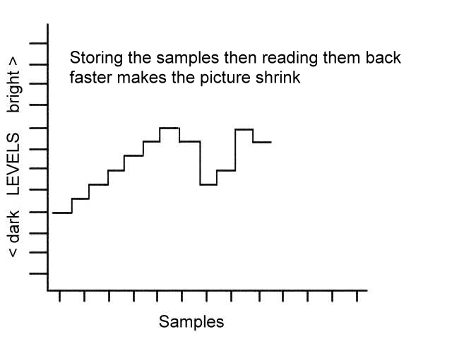
Fig. 6 - compare the waveform width with that in fig. 4a
As you can see, it is possible to perform all sorts of video position and level changing by just tweaking a few numbers. Digital pictures are much more resilient and versatile than their analogue counterparts. The downside to digital is that massive amounts of numbers are produced. In the next part Im going to explain the trick called compression which reduces the volume of digits without appreciably reducing the picture quality.